General Form
There are several ways of representing a conic section. A common representation, however, is to employ a 6-D vector of coefficients \(\vec\theta=(A,B,C,D,E,F)^\top\in\mathbb{R}^6\) that define the inhomogeneous quadratic equation
The quadratic form of the equation can alternatively be defined in terms of a dot product between the coefficients \(\vec\theta\) and the monomials in \(x,y\) given by the vector \(\vec\xi = (x^2,xy,y^2,x,y,1)^\top\) as [KSK16]
\(\vec\xi\) is termed dual-Grassmanian and \(\vec\theta\) Grassmanian coordinates of the conics [HOLearyZM08].
The quadratic equation can be homogenized be substituting \(x'=\frac{x}{w}\) and \(y'=\frac{y}{w}\) for \((x,y)^\top\) [HZ04]. This allows to obtain a symmetric \(3\times3\) matrix that describes the conic. Projective transformations can then be conveniently expressed by matrix products.
- class conics.Conic(*args)[source]
Initializes the conic using the given coefficents.
- Parameters:
args (array_like, optional) – Coeffcients of the quadratic curve.
- property center
Returns the midpoint of a central conic [Ayo93].
- Returns:
2-D coordinate of the conic center.
- Return type:
- constrain(pts, type='parabola', fix_angle=False)[source]
Conditions the conic to a specific type and specific properties.
- Parameters:
pts (numpy.ndarray) – \(n\) 2-D coordinates given by a \(2\times n\) matrix where each coordinate is stored in a column. The conditioning is performed with respect to the specified coordinates.
type (str) – Desired conic type. Possible choice is only
parabola.fix_angle (bool, float) – Specifies whether to fix the angle to the current configuration or use a specific value given by the argument in radians.
- Returns:
The constrained conic.
- Return type:
- static from_circle(x0, r)[source]
Constructs a conic from geometric representation of a circle.
- Parameters:
x0 (array_like) – The 2-D center of the circle.
r (float) – The circle radius.
- Returns:
The circle conic.
- Return type:
- static from_ellipse(x0, major_minor, alpha)[source]
Constructs a conic section from ellipse parameters.
- Parameters:
x0 (array_like) – The 2-D center of the ellipse.
major_minor (array_like) – The size of the half axes.
angle (float) – The orientation of the ellipse in radians.
- Returns:
The ellipse conic.
- Return type:
- static from_homogeneous(Q)[source]
Constructs a conic section from its homogeneous \(3\times3\) symmetric matrix representation.
- Returns:
New conic section
- Return type:
- Raises:
ValueError – Raised if the Q is not symmetric.
- static from_parabola(center, p, alpha)[source]
Constructs a conic section from the geometric representation of a parabola.
The conversion uses the method from [ARW01].
- Parameters:
center (numpy.ndarray) – The 2-D coordinate of the parabola vertex.
p (float) – The distance from the focus.
alpha (float) – Parabola orientation (in radians).
- Returns:
New conic section.
- Return type:
- gradient(pts)[source]
Computes the conic first-order derivative with respect to its coordinates:
\[\begin{split}\nabla Q(x,y) = \left( \frac{\partial Q}{\partial x}, \frac{\partial Q}{\partial y} \right)^\top = \begin{bmatrix} 2Ax+By+D \\ Bx+2Cy+E \end{bmatrix} \enspace .\end{split}\]- Parameters:
pts (numpy.ndarray) – 2-D coordinates where the gradient is evaluated.
- Returns:
The gradient vector with respect to each 2-D coordinate.
- Return type:
- property homogeneous
Returns the homogeneous \(3\times3\) symmetric matrix that represents the conic section. The matrix is given by
\[\begin{split}\tilde{Q} = \begin{bmatrix} A & B/2 & D/2 \\ B/2 & C & E/2 \\ D/2 & E/2 & F \end{bmatrix}\end{split}\]For every point \(\vec p=(x,y,1)^\top\) the quadratic curve can then be expressed by
\[\vec p^\top \tilde{Q} \vec p=0\]
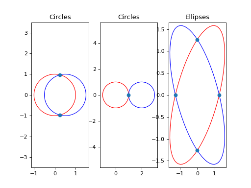
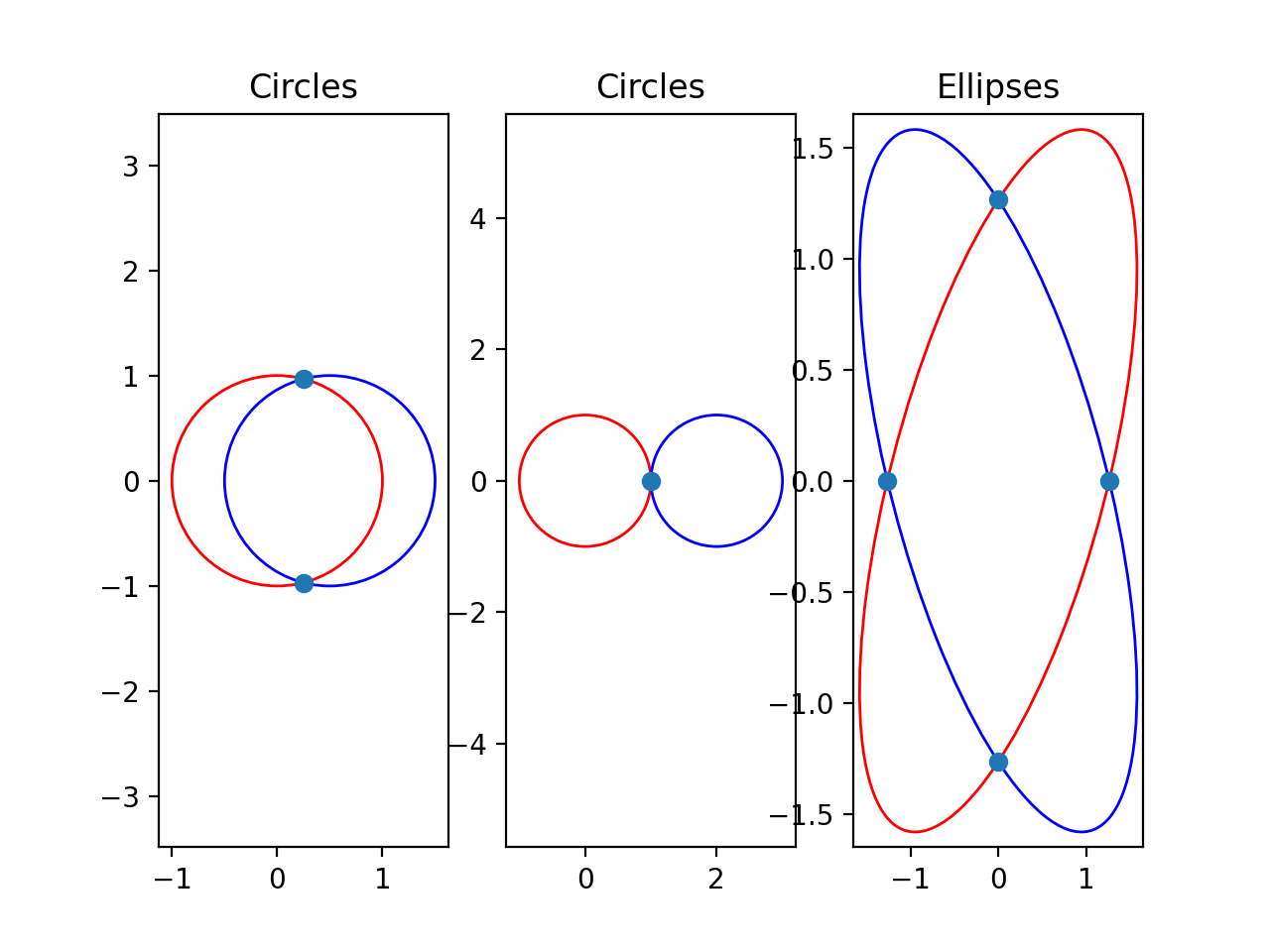
- intersect(other, atol=0.0001)[source]
Computes the intersections of self with another conic.
The method implements the algorithm introduced in [RG11].
- Parameters:
- Returns:
A matrix of homogeneous 2-D points stored in column vectors of a \(3\times N\) matrix consisting of \(0\leq N\leq 4\) columns.
- Return type:
(
Source code,png,hires.png,pdf)
- normalize(d=-1)[source]
Normalizes the conic coefficients such that the determinant of the homogeneous symmetric matrix obtains the specified value d, i.e., \(\det Q = d\) where \(Q\in\mathbb{R}^{3\times3}\) is the conic in the matrix form. The normalization scheme was proposed in [KL93].
To obtain a specific determinant value, one can exploit the determinant property \(\det(kC) = k^n \det C\) where \(n\) is the size of the square matrix. Here, we want to determine the factor \(k\) that yields the desired determinant because
\[k^n \det C=d \iff k^n=\frac{d}{\det C}\]Since \(n=3\), it follows that \(k=\sqrt[3]{\frac{d}{\det C}}\).
- Parameters:
d (float) – The determinant value the matrix form the conic should obtain.
- Returns:
The normalized conic.
- Return type:
- rotate(angle)[source]
Rotates the points on the conic in the counter-clockwise direction.
- Parameters:
angle (float) – The counter-clockwise rotation angle, in radians.
- Returns:
The rotated conic section.
- Return type:
- scale(sx, sy=None)[source]
Scales the conic coordinates.
- Parameters:
- Returns:
Scaled conic.
- Return type:
- to_ellipse()[source]
Returns the geometric representation of the ellipse conic.
- Returns:
A tuple containing the ellipse center \(\vec x_c\in\mathbb{R}^2\), the length of the semi-major and semi- minor axes \((a,b)\in\mathbb{R}_{>0}^2\), and the ellipse orientation \(-\pi\leq\alpha<\pi\).
- Return type:
- to_parabola()[source]
Returns the geometric representation of the parabola given by the current conic.
- Returns:
2-D coordinate \(\vec x_c\in\mathbb{R}^2\) of the parabola vertex, the distance \(p>0\) from the focus and the parabola orientation \(-\pi\leq\alpha<\pi\).
- Return type:
- transform(R, L=None, invert=True)[source]
Transforms the conic using a homography \(H\in\mathbb{R}^{3\times3}\) as
\[\tilde{C}' = (H\vec p)^\top \tilde{C}(H\vec p) = \vec p^\top (H^\top \tilde{C} H) \vec p\]See [HZ04] for details.
- Parameters:
R (numpy.ndarray) – The applied homography on the right hand-side of the original conic section (unless L is given)
L (numpy.ndarray) – The applied homography on the left hand-side of the original conic section. If not given, the transform is computed as the transpose of R.
invert (bool) – Indicates whether the inverse of the homography will be used to transform the conic. Set to True if you intend to transform the points on the conic (default). If False, the transformation is applied as is without inversion.
- Returns:
The transform conic section.
- Return type: