The importance of data normalization

Standardizing point coordinates before performing algebraic fitting can noticeably improve the numerical conditioning of the resulting estimate. This example fits a parabola to points whose coordinate ranges differ substantially between the horizontal and vertical axes, once without scaling and once with scaling enabled, and compares the two results.

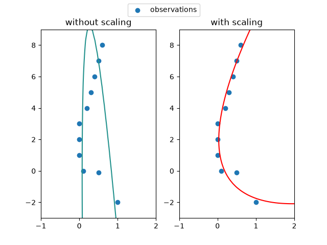
from conics.fitting import fit_nievergelt
import matplotlib.pyplot as plt
import numpy as np

y = [-2, -0.1, 0, 1, 2, 3, 4, 5, 6, 7, 8]
x = [1, 0.5, 0.1, 0, 0, 0, 0.2, 0.3, 0.4, 0.5, 0.6]

pts = np.column_stack((x, y))

C1 = fit_nievergelt(pts, type='parabola', scale=False)
C2 = fit_nievergelt(pts, type='parabola', scale=True)

X, Y = np.meshgrid(
    np.linspace(np.min(x) - 1, np.max(x) + 1),
    np.linspace(-1 + np.min(y), np.max(y) + 1),
)
Z1 = C1(np.dstack([X, Y]))
Z2 = C2(np.dstack([X, Y]))

fig = plt.figure()

ax1, ax2 = fig.subplots(1, 2)

ax1.contour(X, Y, Z1, levels=0)

ax2.contour(X, Y, Z2, colors='red', levels=0)

ax1.scatter(x, y, label='observations')
ax2.scatter(x, y)

ax1.set_title('without scaling')
ax2.set_title('with scaling')

fig.legend(loc='upper center')
plt.show()